![]() We recently showed you how Yoctopuce serial interfaces could make computations on the values read in order to present them directly in a form that the user can use. Today, we show you a similar feature which is also present on some of our analog electrical sensors.
We recently showed you how Yoctopuce serial interfaces could make computations on the values read in order to present them directly in a form that the user can use. Today, we show you a similar feature which is also present on some of our analog electrical sensors.
The sensors that we are going to talk about today are those designed to decode a physical quantity transmitted in the form of an analog signal. They are:
- the Yocto-0-10V-Rx, designed for signals at the 0-10V standard
- the Yocto-4-20mA-Rx, designed for signals at the 4-20mA standard (current loop)
- the Yocto-PWM-Rx, designed for signals encoded by pulse width modulation (PWM) or by variable frequency
- the Yocto-Bridge and the Yocto-MaxiBridge, designed for ratiometric signals
- the Yocto-milliVolt-Rx and the Yocto-milliVolt-Rx-BNC, designed for high impedance signals between -1V and 1V
- the Yocto-MaxiMicroVolt-Rx, designed for the differential measure of low voltages.
The common factor between these sensors is that they present one or several measures with the GenericSensor class.
The GenericSensor class
The sensors of the GenericSensor class share the advantages of all the classes of the Yoctopuce sensors that we described in this previous post. But on top of this, they enable you to
- define a linear correspondence between the value of the measured signal and the corresponding physical quantity
- to freely select the unit advertised by the sensor
Here is what the configuration interface looks like:

GenericSensor configuration interface
Thus, once properly configured, the visible value of a GenericSensor is not the electrical value measured on the sensor, but the corresponding physical quantity. The signal encoding/decoding is managed transparently. Note that you can always read the signal value, if need be, with the get_signalValue() method and you can visualize it in the VirtualHub.
Another specificity of the GenericSensor: you can select among several sampling speeds depending on your needs: either a very fast sampling, or a slower sampling with less noise, or even a sampling filtered by a 5 position median filter. Note that the selection of a sampling speed has no effect on the Yocto-PWM-Rx, as with this module the sampling is always performed at the frequency of the signal itself.
The ArithmeticSensor class
The Yocto-MaxiMicroVolt-Rx proposes an additional possibility to decode a physical quantity based on measured electrical signal: it implements virtuals sensors, using the ArithmeticSensor class, of which you can define the value freely with a mathematic formula with all the sensors of the device. They have the following advantages compared to a GenericSensor:
- they enable you to define a non-linear relation between the measured signal and the physical quantity
- they enable you to combine several measured signals in the computation of a physical quantity
These two characteristics are especially interesting to read electrochemical gas sensors, the use of which generally requires combining the signal produced by an active electrode and an auxiliary electrode to compensate for crossed sensitivity or for temperature drift. Here is a detailed example.
Reading Alphasense electrochemical gas sensors
Alphasense manufactures and commercializes electrochemical gas sensors. You can buy them naked, with an output in nA/ppm rather difficult to read accurately, or mounted by Alphasense on a low noise amperometric circuit with an output in mV/ppb and of which the offset and gain parameters are provided by Alphasense. This later version is the most interesting one as it is easier to acquire measures and as you can simply replace the PCB, sensor included, when the sensor reaches end of life.
Computing gas concentration from mV/ppb signals with integration of the temperature compensation is nevertheless rather complex. Alphasense provides an application note (AAN 803-05) which explains the different proposed compensation methods and provides the corresponding arithmetic formulas. We are therefore going to show you how you can introduce these formulas in the configuration of an ArithmeticSensor, in order to obtain a value that you can directly interpret as a gas concentration. We base this example on sensors NO2-B43F and OX-B431, as they are the most complex due to the crossed sensitivity of the OX-B431 sensor to NO2.
1. We begin by giving a logical name to each input: t for the temperature, NO2_We for the measure on the NO2 work electrode, NO2_Ae for the auxiliary electrode, and so on. These name correspond to those used in the Alphasense application note and this will therefore make our work easier to input the formula in the next step. We also give a name to each arithmeticSensor that we are going to define:

General configuration of the Yocto-MaxiMicroVolt-Rx
2. The configuration of each genericSensor input is trivial: we intentionally keep the signal in mV at this stage, to register it as is in the data logger in case we would like to check the computations later on.

Configuration of the genericSensors
3. Magic comes when configuring arithmeticSensors. We enter almost literally the equation provided by the Alphasense application note, as we can reference the input by their logical name. The expression syntax is the same as the COMPUTE command that we described in a previous post. You can also use arbitrary user-defined function in the formula, such as below the NO2_B43F_N1(t) function which is defined later.

Configuration of the arithmeticSensor1
4. As Alphasense proposes two compensation methods for each sensor, we implement the two methods in two distinct arithmeticSensors in order to compare the results.

Configuration of the arithmeticSensor2
5. For the OX-B431 sensor, the formula is slightly more complex because we must also compensate the crossed sensitivity of the OX sensor with regards to the N02 (see page 3 of the application note). To do so, we use the NO2 measure and we subtract to the input signal in mV the theoretic value generated by the detected NO2. For this reason, it is important to put the NO2-B43F and the OX-B431 sensors on the same Yocto-MaxiMicroVolt-Rx. Note that the factor of crossed sensitivity to NO2 of the OX-B431 should be provided by Alphasense, but it hadn't been communicated to us. A simple email to Alphasense support allowed us to obtain the missing coefficient, as Alphasense keeps in a database the measured coefficients of all the sensors it sells.

Configuration of arithmeticSensor3

Configuration of arithmeticSensor4
6. Background current compensation factors depending on the temperature are provided in tables at the end of the application note. We can enter them in the Yocto-MaxiMicroVolt-Rx as user-defined auxiliary functions, with the button on the bottom of the window for defining arithmetic formulas.

Auxiliary function defined by the user
7. Defining an auxiliary function is performed simply by listing the arbitrary coefficients in a text area. The values between the specified points are linearly interpolated. Here is therefore the definition of the n(t) and k(t) used respectively by methods 1 and 3 of the Alphasense application note, for the NO2 sensor and the OX sensor.
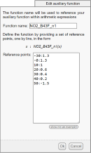
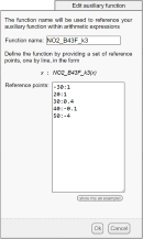
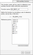
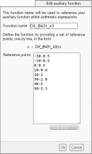
Definition of the temperature compensation coefficients n(t) and k(t)
Results
Because the ArithmeticSensor class behaves like any Yoctopuce sensor, we can display the computed measures directly with Yocto-Visualization:

Measures performed with the OX-B431 sensor
Wee see that Alphasense formulas are a good starting point for temperature compensation, although they cannot compensate for the large warm-up in the morning when the sun warms the sensor. Negative NO2 values should also be filtered. For comparison purposes, here is the reference measure performed by an official station located a few kilometers away:

Reference measures of the Passeiry station

