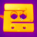
 A rather unique specificity of the Yocto-Bridge, and of its big brother the Yocto-MaxiBridge, is the possibility to perform a software compensation of the temperature drift of the load cell. But is it truly necessary, and how do we go about it? Those are the questions that we are going to answer here.
All serious load cells already include some hardware compensation for temperature, in the shape of thermistors which correct part of the measurement errors caused by variations in temperature. For many applications, this can be enough. Unfortunately, as we are going to see, this hardware compensation doesn't truly cancel the effect of temperature change. Therefore, there is the need for an additional software correction.
When hardware compensation is enough
First observation: we notice that measurement variations caused by temperature changes are usually rather proportional to the temperature. We can therefore admit at once that when you work in an environment where the temperature in controlled, such as an air conditioned room, the problem doesn't exist.
Second observation: the main issue that we observe in case of temperature change is a zero drift. For all applications where you can tare the scale to zero right before the measure, you have already worked around the drift.
These two points cover a large majority of applications with load cells, without having to raise any more questions.
When an additional compensation is required
The problematic situation is therefore when you must weigh an object without being able to tare the scale, in an environment subjected to large temperature variations, typically outside. A typical example is the monitoring of beehives with automatic scales, in order to monitor the activity of the colony and detect a potential hiving-off as soon as possible.
To know if an additional compensation is truly required, you can start by reading the manufacturer's specification sheet. For example, for the small precision scale that we showed you at the end of a previous post, the load cell manufacturer indicates:

For a cell which can weigh up to 300g, a 0.03% * 300g is about 0.1g per 10 degrees of temperature variation. We have therefore put this scale under a protective bell outside, and we activated the data logger of the Yocto-Bridge to see what actually happened over a few days:
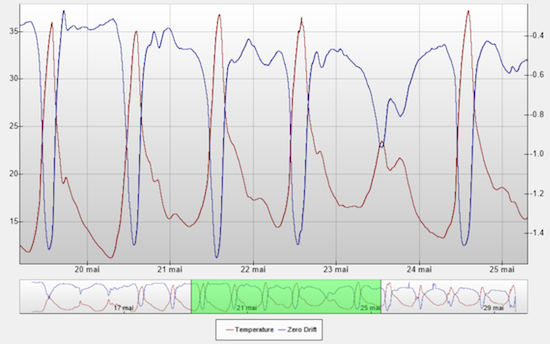
Observed temperature and tare drift
First observation: The tare drift is actually in the order of 0.5g per 10 degrees, and not 0.1g as announced. In case of large day/night temperature variations, this could lead to measurement errors close to 1%, which becomes problematic.
Second observation: As previously mentioned, there is a very strong correlation between the observed error and the temperature, thus the idea to perform a software correction to improve the measure quality. We still need to know which formula to use...
Error modeling
If we examine more closely the correlation between the temperature and the zero drift, we notice that the shape of the curves is not identical. It's therefore not a simple linear dependency. There is therefore a phenomenon causing an indirect fluctuation of the measured dead weight. As we found almost no literature covering this phenomenon, we performed some small numerical experiments and discovered that, on all the load cell in our possession, there were two main components in the error:
- A component which depends linearly on the average temperature
- A component which depends linearly on temperature variations
The dependency on the temperature variation is due to either an asymmetrical propagation of the heat in the load cell, or to an effect delayed in time of the temperature compensation hardware mechanism, causing a differential error. As proof of the existence of this component depending on the change variation, here is the same graph as previously, but this time with temperature variations:
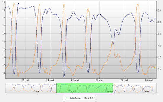
Temperature
The likeness between the curves is striking this time. But to obtain such a good likeness, we had to incorporate a miracle parameter: the cell thermal inertia. Indeed, temperature variations don't impact the cell immediately, the heat needs some time to penetrate the cell. We use a typical formula for heat transmission in a material:

This formula means simply that at each evaluation, the reference temperature for the computation of the compensation is computed as the previous value to which is added a small proportion of the difference between the outside temperature and the current temperature. In our case, we update the temperature every ten seconds, and we use a β factor of about 0.5‰.
Determining the optimal compensation parameters
If you want to subtract as much as possible the measurement error due to the temperature, you need to determine four parameters depending on the whole system and on its thermal inertia:
- The β coefficient of thermal transmission for temperature variation
- The error proportion caused by the temperature variation
- The β coefficient of thermal transmission for the average temperature
- The error proportion caused by the average temperature
The principle consists therefore in installing the measuring system in its native environment, and to record the temperature and the dead weight continuously, in average value 6 times per minute, for one or two weeks. As the Yocto-Bridge is equipped with a data logger and a temperature probe, you can do this very easily with the Yocto-Visualization application. We then save the raw data in a CSV file to use them for the computation.
You then open this file with a small program that we have prepared, and the required parameters are automatically computed, so that you only need to configure them in the Yocto-Bridge.
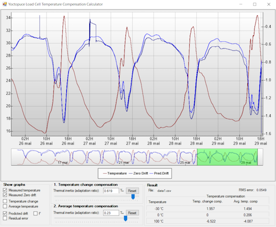
The tool to compute the temperature compensation parameters
Computing method
If you want to know more on the inner workings of this software, available as source code on GitHub, here are a few basic pieces of information.
The first coefficient of thermal transmission for temperature variation is the hardest to compute analytically. We therefore opted to determine it through iterative approximations: we try with a coefficient of 1‰, 0.9‰, 0.8‰ and so on and when we find the best interval, we look for the next decimal.
For a given thermal transmission, it is easy to compute the error proportion to apply. Indeed, as we expect that the zero drift and the temperature variation have identical shapes, their derivative are also identical and both centered on zero. We thus compute the absolute proportion of those two curves, on the basis of their standard deviation, and we know the causality proportion.
To compensate the remainder of the error, depending on the average temperature, we subtract to the measured error the correction depending on the temperature variation, computed previously, and we proceed again in the same way: iterative approximations of the thermal transmission coefficient, and computation of the error proportion with a comparison of the standard deviation.
We tried to see if we could improve the result through a multiple optimization of the parameters with a gradient descent, but the effort is not worth it: the above method already provides a quasi-optimal result for a much lesser cost.
Conclusion: does it work?
The moment of truth consists in comparing the residual error with the original error to see what we actually gain. For the test to be trustworthy, we determine the compensation parameters with the tool only on the first 75% of the measures. Thus, you can observe on the remainder 25% how the system behaves on new measures:
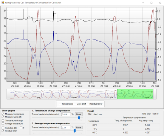
Reducing the obtained error with software compensation
We notice that in the present case, the offset drift could be divided by a factor of about 5 to 10. It's a typical improvement of the results that this method enables you to obtain on different load cells. In many cases, the difference is therefore significant. For example, by looking in details at the graph, we observe a small leap of 0.2g on the measure on May 27, probably caused by a bug which must have landed on the scale pan and stayed there for a few hours. While this leap was mostly hidden by important thermal variations on the original data, it is now clearly visible on the data improved by software compensation.


